This section assumes you have completed Tutorial Part3.

Compare viral loads

In part 3, we compared the viral counts between the two sample groups for Podoviridae, and it appeared as though group B had more viral sequence hits on average than group A. We can compare the normalised counts for these two groups to see if they're significantly different.

Student's T-test

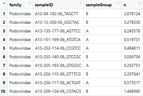
Let's check out the dataframe we made earlier that we'll be using for the test:

View(podoCounts)

We'll use the base-r function t.test(), which takes two vectors--one with the group A counts and one with the group B counts. We can use the filter() and pull() functions within the t.test() function like so:

t.test(
    podoCounts %>% 
        filter(sampleGroup=='A') %>% 
        pull(n),
    podoCounts %>% 
        filter(sampleGroup=='B') %>% 
        pull(n),
    alternative='two.sided',
    paired=F,
    var.equal=T)

    Two Sample t-test

data:  podoCounts %>% filter(sampleGroup == "A") %>% pull(n) and podoCounts %>% filter(sampleGroup == "B") %>% pull(n)
t = -5.3033, df = 8, p-value = 0.0007255
alternative hypothesis: true difference in means is not equal to 0
95 percent confidence interval:
 -615.5267 -242.4563
sample estimates:
mean of x mean of y 
 81.11595 510.10744

Wilcoxon test

You might prefer to perform a Wilcoxon test; the syntax is very similar to the t.test:

wilcox.test(
    podoCounts %>% 
        filter(sampleGroup=='A') %>% 
        pull(n),
    podoCounts %>% 
        filter(sampleGroup=='B') %>% 
        pull(n),
    alternative='t',
    paired=F)

    Wilcoxon rank sum exact test

data:  podoCounts %>% filter(sampleGroup == "A") %>% pull(n) and podoCounts %>% filter(sampleGroup == "B") %>% pull(n)
W = 0, p-value = 0.007937
alternative hypothesis: true location shift is not equal to 0

Dunn's test

Let's use Dunn's test to check all the major families at the same time. Dunn's is good for if you have three or more categories for a metadata field, such as our vaccine column. First find out what the major families are by summing the hits for each family and sorting the table.

# collect the family counts
viralFamCounts = virusesFiltered %>% 
    group_by(family) %>% 
    summarise(n=sum(percent)) %>% 
    arrange(desc(n))

# update factor levels to the sorted order
viralFamCounts$family = factor(viralFamCounts$family,levels=viralFamCounts$family)

and plot:

ggplot(viralFamCounts) +
    geom_bar(aes(x=family,y=n),stat='identity') +
    coord_flip()

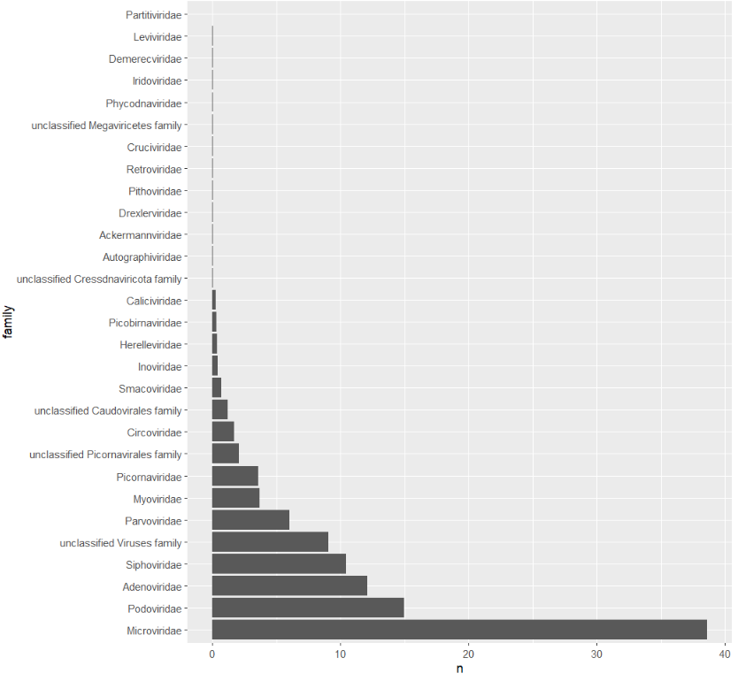
Let's focus on Siphoviridae, Adenoviridae, Podoviridae, and Microviridae. Collect summary counts for these families for each sample and include the metadata we want to use:

viralMajorFamCounts = viruses %>% 
    filter(family %in% c('Siphoviridae','Adenoviridae','Podoviridae','Microviridae')) %>% 
    group_by(sampleID,family,vaccine) %>% 
    summarise(n=sum(percent))

Now let's do the dunn's test for these families:

viralMajorFamCounts %>% 
    group_by(family) %>% 
    dunn_test(n ~ vaccine,p.adjust.method='holm') %>% 
    add_significance()

# A tibble: 12 × 10
   family       .y.   group1     group2        n1    n2 statistic      p  p.adj p.adj.signif
 * <chr>        <chr> <chr>      <chr>      <int> <int>     <dbl>  <dbl>  <dbl> <chr>       
 1 Adenoviridae n     Ad_alone   Ad_protein     3     2     0.467 0.641  1      ns          
 2 Adenoviridae n     Ad_alone   sham           3     4     0.438 0.661  1      ns          
 3 Adenoviridae n     Ad_protein sham           2     4    -0.105 0.916  1      ns          
 4 Microviridae n     Ad_alone   Ad_protein     4     2    -1.43  0.153  0.458  ns          
 5 Microviridae n     Ad_alone   sham           4     4    -0.584 0.559  0.681  ns          
 6 Microviridae n     Ad_protein sham           2     4     0.953 0.340  0.681  ns          
 7 Podoviridae  n     Ad_alone   Ad_protein     4     2     0.477 0.634  0.681  ns          
 8 Podoviridae  n     Ad_alone   sham           4     4     1.75  0.0798 0.240  ns          
 9 Podoviridae  n     Ad_protein sham           2     4     0.953 0.340  0.681  ns          
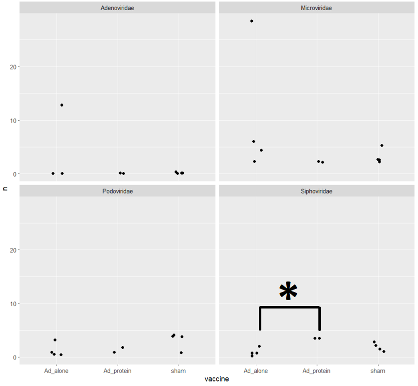
10 Siphoviridae n     Ad_alone   Ad_protein     4     2     2.48  0.0132 0.0395 *           
11 Siphoviridae n     Ad_alone   sham           4     4     1.40  0.161  0.322  ns          
12 Siphoviridae n     Ad_protein sham           2     4    -1.33  0.182  0.322  ns

There's only one comparison that is significant. Let's put it on a plot

ggplot(viralMajorFamCounts) +
    geom_jitter(aes(x=vaccine,y=n)) +
    facet_wrap(~family)

Compare presence/absence

You might not care about viral loads and instead are just interested in comparing the presence or absence of viruses. For this you could use a Fisher's exact test. To perform this test you need to assign a presence '1' or absence '0' for each viral family/genus/etc for each sample. What number of hits you use for deciding if a virus is present is up to you.

I want to be sure about the alignments, so I'll apply some stringent filtering cutoffs. Then I'll assign anything with any hits as 'present' for that viral family. Let's look at Myoviridae ... for no particular reason.

# apply a stringent filter
virusesStringent = viruses %>% 
    filter(evalue<1e-30,alnlen>150,pident>75,alnType=='aa')

# count hits for Myoviridae and score presence
# NOTE: the absent samples WONT be in the table yet, we have to add them in after
myovirPresAbs = virusesStringent %>% 
    filter(family=='Myoviridae') %>%
    group_by(sampleID) %>% 
    summarise(n=sum(percent)) %>%
    mutate(present=ifelse(n>0,1,0))

# merge in the metadata
# Using all=T will do an outer join and bring in the absent samples
myovirPresAbs = merge(myovirPresAbs,meta,by='sampleID',all=T)

# convert na's to zeros
myovirPresAbs[is.na(myovirPresAbs)] = 0

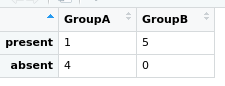
To do the Fisher's exact test we need to specify a 2x2 grid; The first column will be the number with Myoviridae for each group. The second column will be the numbers without for each group.

# matrix rows
mtxGroupA = c(
    myovirPresAbs %>% 
        filter(sampleGroup=='A',present==1) %>% 
        summarise(n=n()) %>% 
        pull(n),
    myovirPresAbs %>% 
        filter(sampleGroup=='A',present==0) %>% 
        summarise(n=n()) %>% 
        pull(n))
mtxGroupB = c(
    myovirPresAbs %>% 
        filter(sampleGroup=='B',present==1) %>% 
        summarise(n=n()) %>% 
        pull(n),
    myovirPresAbs %>% 
        filter(sampleGroup=='B',present==0) %>% 
        summarise(n=n()) %>% 
        pull(n))

# create the 2x2 matrix
myovirFishMtx = matrix(c(mtxGroupA,mtxGroupB),nrow = 2)

# this bit is not necessary, but lets add row and col names to illustrate the matrix layout
colnames(myovirFishMtx) = c('GroupA','GroupB')
row.names(myovirFishMtx) = c('present','absent')

# view
View(myovirFishMtx)

# Run Fisher's exact test
fisher.test(myovirFishMtx)

    Fisher's Exact Test for Count Data

data:  myovirFishMtx
p-value = 0.04762
alternative hypothesis: true odds ratio is not equal to 1
95 percent confidence interval:
 0.000000 0.975779
sample estimates:
odds ratio 
         0

We don't have many samples, so our significance won't be great regardless.

In Part 5 we will look at the contigs' read-based annotations.